This article is still work in progress!
The notes on this page are taken from:
Udacity: Intro to Statistics.
Packt: Statistics for Data Science and Business Analysis .
Population and Sample
Population
- all items of interest
- properties of interest: parameters
- mathematical symbol:
Sample
- a subset of the population
- properties of interest: statistics
- mathematical symbol:
A sample needs to be random and representative for the population.
Data
Types of Data
- Categorical
- Numerical
- Discrete
- Continuous
Measurement Levels
- Qualitative
- Nominal
- Ordinal
- Quantitative
- Interval
- Ratio
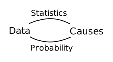
Statistics and Probability
Independent Events
- Probability of Event:
- Probability of opposite Event:
- Probability of composite Events:
Dependent Events
: Probability of Event when already occurred.
Probability Distributions
In Continuous Distributions every outcome has the Probability .
Density
PDF: Probability Density Function
Probability for continuous spaces. Density can be bigger than .
Density:
- Always non-negative
- Doesn’t need to be continuous
- Doesn’t need to be smaller or equal than one
- Integrates to one
Estimation
Estimation problem is:
Data → P
P → P(Data)
Maximum Likelihood Estimator (MLE):
The sum is always between and .
Laplace Estimator:
: Number of Outcomes
: Number of Experiments
Averages
Mean
Sum up all elements and divide by the number of elements.
Population
Sample
Median
Sort all elements and take the one in the middle (or the mean of the two elements in the middle).
- if is odd:
- if is even:
Mode
The value of the elements that appears most often in a data set.
Asymmetry
Skewness
- Positive skew:
- Zero skew:
- Negative skew:
Sample Skewness
Variability
Variance
The variance measures the dispersion of data points around their mean.
Subtract the mean from every item. Then sum up the squares of the subtractions and divide the result by the number of data items.
Population
Sample
Standard Deviation
The standard deviation is giving a sense how far away the items in a data set are from the mean.
It is the square root of its variance.
It’s the most common measure of variability for a single data set.
Population
Sample
Coefficient of Variation
It is used to compare multiple data sets.
Population
Sample
Overview of Mean, Variance and Standard Deviation
These notes are taken from Khan Academy
| Concept | Population | Samples |
|---|---|---|
| Mean | ||
| Variance | ||
| Standard Deviation |
: Number of items in Population
: Number of items in sample set taken from the population
For an unbiased estimator (Variance of samples) the sum is divided by !
: is not an unbiased estimator due to the non-linear nature of the square root.
Relationship between Variables
Correlation: variables are statically related.
Covariance
Main statistic to measure correlation.
Population:
Sample:
Correlation Coefficient
Adjust covariance to be easy to interpret.
The correlation coefficient is between and .
Population:
Sample:
Binomial Coefficients
Choose elements from possible elements (without putting back elements and without caring about the order of the chosen elements):
Inferential Statistics
Use Probability Theory and Distributions with sample data, to predict population values.
Distributions
A distribution is a function that shows how often each value of a variable occurs.
Binomial Distribution
Binomial Distribution is a discrete distribution.
i.e. Flip a loaded coin:
: Probability to get a head from one coin flip.
Flip coin times.
: Expectation to get heads from all the flips.
The Normal Distribution
Also called Gaussian Distribution or Bell Curve.
Notation:
Where:
- : Normal Distribution
- : Mean
- : Variance
- : Standard Deviation
Definition:
The expression is needed to normalise the area underneath the curve given by the rest of the formula (). Otherwise, it would not add up to .
Properties:
- mean median mode
- no skew
Standard Normal Distribution
Standardizing the Normal distribution to have a mean and standard deviation .
Formula:
Where:
- : Standard Normal Distribution (-Score)
- : Mean
- : Standard Deviation
Central Limit Theorem (CLT)
Given a normalized sample mean. That is the mean of a number of samples from a population. That sample mean converges to a standard normal distribution as the number of samples increase.
- take a sample from the population
- calculate the mean of that sample (sample mean)
- repeat until enough samples were processed
All the sample means together form the Sampling Distribution of the mean.
The Sampling Distribution of the mean will approximate a normal distribution no matter of what kind the population distribution is (binomial, exponential, …).
Sampling distribution:
The sampling distribution has the same mean as the original (population) distribution. It’s variance is the population variance divided by the sampling size:
Where:
- : mean of the population distribution
- : variance of the population distribution
- : number of samples
Typically, at least around 30 samples are needed for the CLT to apply.
Standard Error
The standard deviation of the sampling distribution.
That is standard deviation of the distribution formed by the sampling mean.
It shows the variability of the means of the samples.
Variance of the sampling distribution:
Standard error:
Estimators
Approximation of a population parameter. Depending on sample information only.
An estimator is a type of (sample) statistic.
A value of an estimator is called estimate. There are:
- point estimates
- confidence interval estimates
The point interval is located in the middle of the confidence interval.
Some basic estimates:
- Sample mean is a point estimate of the population mean .
- Sample variance is a point estimate of the population mean .
Properties of Estimators
- Efficiency
- Bias
Prefer most efficient, unbiased estimator.
Unbiased estimator: expected value equal to population parameter.
Most efficient estimator: unbiased with the smallest variance
Bayes’ Rule
See also Wikipedia
Prior Probability & Test Evidence -> Posterior Probability
Prior:
Posterior:
- : the prior, is the initial degree of belief in .
- : the posterior, is the degree of belief having accounted for .
- the quotient represents the support provides for .
Algorithm
Imagine there is a disease. The possibility to get this particular disease is .
There is a test to check if someone has that disease. But the test is not completely reliable.
Prior: Sensitivity: Specificity:
The Prior says how many people have the disease.
The Sensitivity says how many get a positive test if they have the disease.
The Sensitivity says how many get a negative test if they don’t have the disease.
Imagine someone get’s a positive test result. How can we calculate the probability that this person has the disease?
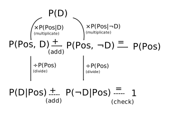
- Take the Prior and multiply it with (Sensitivity) → .
- Take the Prior and multiply it with → .
- Add the results of 1. and 2. up → .
- Divide the result from 1. by the result of 3. → .
- Divide the result from 2. by the result of 3. → .
- Check: add the results of 4. and 5. → .
Note:
The calculation for a negative test result are analogous. Just replace with .