0. Overview
- Specification and Models of Computation
- State-Charts
- Kahn Process Networks
- Design Space Exploration
- Mapping
- Partitioning
- Multi-Criteria Optimization
- Performance Estimation
- Simulation-based Methods
- Worst-Case Execution Time Analysis
- Performance Analysis of Distributed Systems
- Thermal-aware Design
1. Introduction
System Design
- Specifications and Models
- Design
- Estimation
Embedded Systems
- Information processing system embedded in a larger product
- Interface to outside world
- external process
- Sensors, actors
- Human interface
- Technical environment does not forgive errors
- Stricter requirements (usually update not possible)
Difference Embedded Systems ↔ General Purpose Computing
| Embedded Systems | General Purpose Computing |
|---|---|
| Few Applications, known at design-time | Broad class of applications |
| Not programmable by end user | Programmable by end user |
| Fixed run-time requirement | Faster is better |
Levels of abstraction (from higher to lower)
- Transistors
- Gates
- Processor (Memory, Register, ALU, …)
- Architecture (CPU, ASIC, FPGA, LAN, …)
- Distributed System
Design
- Design aspects look similar in every level
- Design goes usually from higher abstraction level to lower level
- Abstraction: leave out (unimportant) details
- System level design:
- SW Synthesis (compile)
- HW Synthesis
- Interfaces
Estimation
- Reason about solution
- Different solutions for a specific task
- Precision of estimation is different on each level
- Higher level estimation usually less precise than lower level
Mapping
- Mapping parts of specification to different parts of the system
- Similar to scheduling but bigger design space (including HW)
Specification
- Specification: in embedded systems higher requirements to correctness
- Specific languages:
- Developer is restricted (lesser errors)
- Better code generator/synthesizer
Doing things right is difficult!
- Observer Pattern is not save!
- Race conditions
- Dead-Locks
- Use non-locking algorithms!
2. Models of Computation
Model of computation = Components + Communication
- Hierarchy
- Behavioral
- Structural
- Timing
- State oriented behavior (micro controller, FPGA)
- Dataflow oriented behavior (DSP)
State Charts
-
Classical automata (Moore/Mealy): FSM
-
State: Information needed to get (determine) the output form the input
-
State Charts introduce hierarchy
- Combining States with Sub-States in Super-States
- Active States
- Basic States (no Sub-States)
- Super-States (ancestor states): OR-Super-States (hierarchy)
- Default State, History State (can be combined)
- AND-Super-States (concurrency)
-
2 distinct features form FSM
- Hierarchy
- Difference of Control-Path and Data-Path
-
Communication between Control- and Data-Path
- Control-Path to Data-Path: action
- Data-Path to Control-Path: condition
-
Events, Conditions, Actions
- No storage of events (only available for next step)
- Events are global
Evaluation of State Charts
- Evaluation is not trivial!
- Three phases
- Event is emitted
- Transition is selected
- Simultaneously make transition and apply the actions
- Execute the right hand side of action simultaneously and assign then after
Specification and Description Language (SDL)
- Targeted at unambiguous specification and description of systems
- Asynchronous message passing
- Appropriate also for distributed systems
- Communication between FSMs (or processes)
- message passing with FIFO queues
- FIFOs can be indefinitely large
- Each process fetches entry from FIFO
- if input enables transition it takes place
- otherwise discard input
- All orders of events are legal: different correct behavior in simulators (not deterministic)
Dataflow Languages
-
Imperative language style (program counter)
-
Movement of data is priority
-
Scheduling: responsibility of the system (not the programmer)
-
Basic characteristics:
- all processes run ‘simultaneously’
- Processes can be described with imperative code
- Processes can only communicate through buffers
- Sequence of read tokens is same as of read tokens
-
Useful for applications that deal with streams of data
- Concurrent: maps to parallel hardware
- Perfect for block-diagram specifications (control systems, signal processing)
Kahn Process Networks
- General-purpose scheme for parallel programming
- read: destructive and blocking (reading empty channel blocks until data is available)
- write: non-blocking
- FIFO: infinite size
- Unique attribute: determinate
Determinacy
- Random: knowing about system and inputs is not sufficient to determine output
- Determinate: the histories of all channels depend only on the histories of the input channels
- Importance
- Functional behavior is independent of timing (scheduling, communication time, execution time of processes)
- Separation of functional properties and timing
Adding Non-Determinacy
- Several possibilities
- Allow processes to test for empty queues
- Allow multiple processes to write to or read from one channel
- Allow processes to share a variable (memory)
Synchronous Dataflow (SDF)
- Restriction of Kahn Networks to allow compile-time scheduling
- Each process reads and writes a fixed number of tokens each time it fires
- Firing is an atomic process
- Schedule can be determined completely at compile-time
- Steps:
- Establish relative execution rates (solving a system of linear balancing equations)
- Determine periodic schedule by simulating system for a single round
3. Mapping Application to Architecture
System synthesis from specification
- Allocation: Select components (HW)
- Binding: Bind SW (Application) to HW (Components)
- Scheduling: Executing code
Mapping = Binding + Scheduling
Specification Examples
Data-Flow Graph (DFG)
x = *3a + B*b - c;
y = a + b*x;
z = b - c*(a + b);- no loops
- parallelism
Control-Flow Graph (CFG)
what_is_this {
    read(a, b);
    done = FALSE;
    repeat {
        if (a>b)
            a = a-b;
        else if (b>a)
            b = b-a;
        else done = TRUE;
    } until done;
    write(a);
}- State machine
- Conditional branches
Control Flow Graph on Wikipedia
Architecture Specification
- Reflects structure and properties of underlying platform
- Can be done at different abstraction levels
Mapping Specification
Mapping: application and architecture specification
- binds processes to processors
- binds communication between processes to architecture communication paths
- specifies resource sharing and scheduling

4. System Partitioning
Partitioning: Given a set of objects: Partition this set in subsets.
Mapping: Subset is mapped to specific resource.
Mapping at different Levels
Low Level
- Register Transfer Level (RTL) or Netlist Level
- Split a digital circuit and map it to several devices (FPGAs, ASICs)
- System parameters (e.g., area, delay) relatively easy to determine
High Level
- System Level
- Comparison of design alternatives for optimality (design space exploration)
- System parameters are unknown and difficult to determine
- to be estimated via analysis, simulation, (rapid) prototyping
Cost Functions
- system cost (C[$])
- latency (L[sec])
- power consumption (P[W])
- …
Estimation
Estimation is required to find C, L, P values, for each design point
i.e
- , , : denote how strong , , violate design constraints , ,
- , , : weighting and normalization
The Formal Partitioning Problem
Assign objects to blocks (also called partitions) , such that
- (all objects are assigned - mapped)
- (an object is not assigned or mapped twice)
- and costs are minimized
Partitioning Methods
Exact vs. Heuristic Methods:
- Exact provides optimal solution (or set of solutions)
- Heuristic provides a ‘good’ solution but not best
Overview:
- Exact Methods
- Enumeration
- Integer linear programs (ILP)
- Heuristic
- Constructive Methods
- Random mapping
- Hierarchical clustering
- Iterative methods
- Kerninghan-Lin algorithm
- Simulated annealing
- Evolutionary algorithm
- Constructive Methods
Hierarchical Clustering
- Combine always 2 nodes
- Then recalculate
- Repeat until goal achieved
- Steps can be visualized in a tree diagram
Integer Linear Programming (ILP)
- Exact method
- Objective function
- Constraints
Objective:
Constraints:
Integer programming problem:
- Minimize objective function subject to constraints
Example for Partitioning
- optimize for a load balanced system
Scheduling:
| Task | t0 | t1 | t2 | t3 |
|---|---|---|---|---|
| Processor0 | 1 | 1 | 0 | 0 |
| Processor1 | 0 | 0 | 1 | 1 |
Run Times:
| Run time | t0 | t1 | t2 | t3 |
|---|---|---|---|---|
| Processor0 | 5 | 15 | 10 | 30 |
| Processor1 | 10 | 20 | 10 | 10 |
Cost :
Binary variables :
Approaches
- Approach:
2. Approach:
This is not a linear problem!
Solutions
1. Solution:
Solving 2 linear problems: split approach 2 into 2 linear problems:
Becomes:
2. Solution:
Empirical approach: Run code and measure execution time and try to minimize it.
Move tasks to different processors.
Iterative Methods
Often used principle:
- Start with some initial configuration (partitioning)
- search neighborhood (similar partitions)
- select a neighbor as candidate
- evaluate fitness (cost) function of candidate
- accept candidate using acceptance rule
- if not, select another neighbor
- Stop if:
- Quality is sufficient or
- no improvement can be found or
- after a fixed time
Ingredients:
- initial configuration
- function to find a neighbor as candidate
- cost function
- acceptance rule
- stop criterion
Disadvantages:
- local optimum as best result
- local optimum depends on initial configuration
- generally no upper bound on iteration length
Kernighan-Lin
- as long as a better partition is found
- from all possible pairs of objects: virtually re-group the ‘best’ (lowest cost of resulting partition)
- from the remaining (not yet touched) objects: virtually re-group the ‘best’ pair
- continue until all objects have been re-grouped
- from these n/2 partitions, take the one with smallest cost and actually perform the corresponding re-group operation
Simulated Annealing
- inspired by physical process
- replace existing solutions by (random) new feasible solutions form neighborhood
- always accept better solutions but allow for a guided acceptance for worse neighbors
- gradually cooling: gradually decrease the probability of accepting worse solutions
Advantage:
- Allowance for ‘uphill’ moves potentially avoids local optima
Possible implementation:
temp = temp_start
cost = c(P)
while Frozen() == False:
    while Equilibrium() == False:
        P_new = RandomMove(P)
        cost_new = c(P_new)
        deltacost = cost_new - cost
        if Accept(deltacost, temp) > random(0,1)
            P = P_new
            cost = cost_new
        temp = DecreaseTemp(temp)
Functions:
RandomMove(P):
- Choose a random solution in the neighborhood of
P
DecreaseTemp(), Frozen():
- Cooling down. There are different choices. For example:
- initially:
temp := 1.0 - in any iteration:
temp := alpha * temp(typically: 0.8alpha0.99)
- initially:
- Frozen
- after a given time or
- if there is not further improvement
Equilibrium():
- Usually after a defined number of iterations
Accept(deltacost, temp):
Complexity:
- From exponential to constant depending on
Equilibrium(), DecreaseTemp() and Frozen().
5. Multi-Criteria Optimization
Part of system synthesis.
Exploration of different solutions.
Example: Network Processors
Network processor: High-performance, programmable device designed to efficiently execute communication workloads
- Given:
- Specification of the task structure (task model): tasks to be executed for each flow
- Different usage scenarios (flow model): sets of flows
- Sought:
- Network processor implementation: architecture + task mapping + scheduling
- Objectives:
- Maximize performance
- Minimize cost
- Subject to:
- Memory constraint
- Delay constraint
Basic Definition
- We intend to minimize a vector-valued objective function
- denotes the decision space. i.e the feasible set of alternatives for the optimization problem
- The image of the decision space using the objective function is denoted as the objective space with
- A single alternative is (sometimes) named solution and the corresponding object value is named objective vector
decision space → objective space
Basic question:
How do we define the minimum of a vector-valued function?
Pareto Dominance
Definition:
A solution weakly Pareto-dominates a solution , denoted as , if it is at least as good in all objectives, i.e:
- Dominance is transitive
- A solution is named Pareto-optimal, if it’s not Pareto-dominated by any other solution in
Optimization Alternatives
- Classical single objective optimization methods
- Simulated annealing
- Integer linear program
- other constructive or iterative heuristic methods
→ Decision making is done before the optimization
- Population based optimization methods
- Evolutionary / genetic algorithms
→ Decision making is done after the optimization
Evolutionary Algorithms
Basic scheme (many variations exist):
- A set of initial solution (initial population is chosen (usually at random). This set is called parent set.
- Solutions form parent set are selected (mating selection)
- Solutions from mating selection are changed using neighborhood operators (cross-over and mutation operators). The resulting set is called children set.
- Determine union of the parent and the children sets
- Solutions of the set from 4. are selected based on their merit to construct the new parent set (environmental selection).
- continue at 2.

- Cross-over operator: Take best parts of two solutions
- Mutation operator: same as in simulated annealing (make small variations)
- How to choose solutions that should be removed from the population
- Solutions should be ‘close’ to the (unknown) Pareto-optimal front (optimality)
- Solutions should cover large parts of the objective space (diversity)
Hypervolume Indicator
- Environmental selection:
- Select subset of solutions that maximizes hypervolume indicator
Given a set of solutions and a set of reference points . Then the hypervolume indicator of with respect to is defined as
where id the dominated space of regarding :
: Objective
- The hypervolume indicator leads to diversity and optimality
Representation and Neighborhood
- A representation corresponds to an abstract data that encodes a solution
- Neighborhood operators work on representations
Issues:
- Each solution has an encoding (completeness)
- All solutions are represented equally often (uniformity)
- Each encoding maps to a feasible solution (feasibility)
Encoding: i.e order of tasks executing to explore scheduling.
Tree Representation
- Solutions can be represented as tree structures
- Mutation:
- Grow subtree
- Shrink subtree
- Switch two subtrees
- Replace subtree
- Subtrees can be single nodes
Handling Constraints
Constraint:
- Feasible:
- Infeasible:
Approaches:
- Representation is chosen such that decoding always yields a feasible solution
- Construct initialization and neighborhood operators such that Infeasible solutions are not generated
- Add only feasible solutions to children population
- Preferably select feasible solutions in environmental selection
- Penalty function:
- Calculate constraint violation and incorporate it into objective function
- i.e add penalty function to every objective (increase ‘price’ for Infeasible solutions)
- Include the constraints as new objectives
6. System Simulation
Estimation with simulation.
Estimation: find out if a solution is good or bad.
System and Model
- System: Combination of components that act together
- Model: Formal description of the system (covers selected information)
State
- Contains all information of the system at that is necessary to determine the output (for ) from the input (at (at ).
Input + State = Output
- The set of all possible states of a system is called it’s state space
Discrete/Continuous Systems
Examples:
- Continuous state systems:
- Physical processes (usually)
- Electrical networks
- Mechanical systems
- Discrete state systems
- Finite state machines
- Queuing systems
- Computer systems
- Continuous time systems
- Physical processes (usually)
- Electrical circuits
- Asynchronous systems
- Discrete time systems
- Digital clocked system
- Equidistant sampling (z-transform)
- Synchronous system models
Discrete Event Systems (DES)
-
Driven by events
-
Event: is a touple of a value and a tag
- Tags are usually totally ordered
- If the tag denotes time, then the event is a timed event
- If the tag (only) denotes a sequence number, the event is an untimed event
-
DES is an event-driven system
- Depends entirely on occurrence of discrete events
- Does not depend on evolution of time
-
Can be defined in continuous of discrete time
-
The state space can be either discrete or continuous
-
Signals or streams represent ordering/timing of events
-
Processes are represented as functions acting on signals or streams
Simulation
-
Discrete-time, time-driven
- Simulated time is partitioned into equidistant time intervals
- Length of time intervals determined by
- The simulated system (i.e clock period)
- The intended precision (dicretization loss)
- The simulation effort
- A simulation step is performed even if nothing happens
-
Event-driven simulation
- State change only at events
- Analysis and simulation possible in discrete or continuous time
Discrete-Event Modeling and Simulation
- Concurrent processes are modeled using modules
- Behavior described as logic/algebraic expressions
- State described using persistent variables (inside module)
- Communication between modules through ports, via signals
- Synchronization through abstract events
- Modules can be hierarchical
- Event-Driven
Components of Discrete-Event Simulation
- Simulation time
- Simulation clock represents the current value of simulation time
- In discrete-event simulations the clock advances to the next event start-time during simulation
- Event list
- Events are processed in order
- Event list is typically organized as priority queue
- Event lists may include simulation times when events will happen
- System modules
- Model subsystems of simulated system
- Are called by simulation engine if a relevant event is scheduled
Simulation Engine
- Initialization routine
- Initialize the simulation model;
- Set initial states of subsystem modules
- Fill the event queue with initial events
- Initialize the simulation model;
- Timing routine
- Determine next event from the event queue
- Advance the simulation clock to the time when the event occurs
- Event routine
- Update system state when event occurs
- In a simulation cycle ‘cause’ and ‘effect’ can share the same time of occurrence
- Use zero duration virtual time interval called delta cycle ()
SystemC
- System-level modeling language
- Several levels of abstractions
- from purely functional
- to cycle-accurate/pin-accurate
- Special attention to systems with embedded software
- Several levels of abstractions
- C++ library for modeling concurrent systems
- HW-oriented data types
- Communication mechanisms
- Concurrency modeling
- Event-driven simulation kernel for executing models
- Free (open source)
- For Windows, Linux, OS X…
Language Architecture
- Core language
- Minimal set of modeling constructs
- structural description
- concurrency
- communication
- synchronization
- Minimal set of modeling constructs
- Data types (separated from core language)
- On top of core language
- Communication mechanism (signals, FIFO…)
- Models of Computation (MoCs)
- Layer (tier) architecture
Processes
Processes are the basic units of functionality.
SC_THREADs- Typically called once, run forever (in a
while(true)loop) - Can be suspended by calling
wait() - Keep the state of execution implicitly
- Typically called once, run forever (in a
SC_METHODs- Execute repeatedly from the beginning to end
- Simulate faster
- Do not keep the state of execution implicitly
- Processes must be contained in a module
- Bun not every member function is a process
Modules
- Building blocks of models
- Hierarchy
- Abstraction
- IP reuse
Inter Process Communication
- Processes can communicate directly trough signals
- Events: Flexible, low-level synchronization primitive
- Channel:
- Container for communication and synchronization
- can have state (private data), transport data, transport events
- Implement one or more interfaces
- Container for communication and synchronization
- Interface:
- Set of access methods to the channel
- Interface methods need to be implemented
Wait and Notify
wait: halt process until an extent is raisedwait()with arguments → dynamic sensitivitywait(sc_event)wait(time)wait(timeout, sc_event)
notify: rise an eventnotify()with arguments → delayed notificationmy_event.notify();: notify immediatelymy_event.notify(SC_ZERO_TIME);: notify next delta cyclemy_event.notify(time);: notify after ‘time’
Levels of Abstractions
Simulation can be done on different levels of abstraction.
- Functional level (untimed/timed)
- Use: Model (un-)timed functionality
- Communication: shared variables, messages
- Typical languages: C/C++, Matlab
- Transaction level
- Use:
- MPSoC architecture analysis
- Early SW development
- Timing estimation
- Communication: method calls to channels
- Typical languages: SystemC
- Use:
- Register transfer level / Pin level
- Use: HW design and verification
- Communication: wires and registers
- Typical languages: Verilog, VHDL
7. Design Space Exploration
Example: Network Processor (NP)
- Different processing units: ARM9, DSP, …
- Streams: ordered sequence of tasks
Optimal Design of Network Processor
: Tasks : Requests : Mapping : Resources : Cost
- Mappings: all possible bindings of tasks
- i.e if then task could be executed on resource
- Request
- i.e execution of one packet in would use computing units of
- Resource allocation cost
- Binding of tasks to resources
- leading to actual implementation
- Subset of mappings s.t every task is bound to exactly one allocated resource
- and
Design constraints
- Delay constraints: e.g max time a packet is processed within network processor
- Throughput maximization: e.g packets per second
- Cost minimization: implementing with small amount of resources (processing units, memory, networks…)
- And conflicting usage scenarios …
NP Design Space Exploration
- Allocation: determine HW components
- Binding: For each SW process choose allocated HW unit
- Scheduling: For tasks on specific resources choose scheduling policy
Performance Estimation
Global Picture
Metric
- Time
- Power
- Area (integration on silicon)
- Cost
- Quality
- SNR
- …
Method
- Analytic
- Simulation
- Statistic
Abstraction Level
- Low-level: Register Transfer Level, Instruction Set Architecture
- Intermediary-level: Transaction Level-Model, Operating System, already linked to HW
- High-level: Functional, High-level language, independent of HW
Subsystem to Analyze
- HW subsystem
- CPU subsystem
- Interconnect subsystem
- Multiprocessor System-on-Chip (MPSoC)
Performance Estimation in Design Flow
- High-level
- Advantages:
- Short estimation time (fast)
- Implementation details not necessary
- Drawbacks:
- Limited accuracy
- e.g no information about timing
- Advantages:
- Low-level
- Advantages:
- Higher accuracy
- Drawbacks:
- Long estimation time (slow)
- Many implementation details need to be known
- Advantages:
Multi-Processor System-on-Chip
Simulation should be divided in to independent modules. So they can be exchanged.
Composable in terms of:
- Subsystems
- Interactions
- Computation
- Communication
- Memory
- Scheduling
Estimation should cover different metrics e.g:
- Delays
- Throughput
- Memory consumption
- Power
- Energy
- Temperature
- Cost
- …
Communication
- Bus
- Network
- Hierarchical Bus
Computation and Memory
- DRAM
- SDRAM
- DSP
- RISC
- FPGA
- muC
- HW
Scheduling and Arbitration
- TDMA
- EDF
- FCFS
- proportional share
- fixed priority
- static
Difficulty
Why is MPSoC performance estimation difficult?
- Computation, communication and memory
- Non-deterministic computation in processing nodes
- Non-deterministic communication delays
- Non-deterministic memory access
- Complex resource interaction via scheduling/arbitration
- Cyclic timing dependencies
- Internal data streams interact on computation and communication resources
- Interaction determines stream characteristics
- Uncertain environment
- Different load scenarios
- Unknown, worst case inputs
Making one component faster can make the complete system slower!
If a component is replaced with a faster one it could block shared resources (e.g bus) for other components.
Abstraction
- Technology: transistors, layouts
- Signal: gate, schematic, RTL
- Transaction: SW, HW systems
- Tokens: SW tasks, comm. backbones, IPs
- Simulators:
- SPICE
- VHDL
- SystemC / Instruction Set Simulator
- …
Performance Estimation Methods
How to evaluate a system?
- Measurements
- Use existing instance of the system to measure performance
- Simulation
- Develop a program which implements a model of the system and evaluate performance by running the program
- Statistics
- Develop a statistical abstraction of the system and derive statistic performance via analysis or simulation
- Formal analysis
- Develop a mathematical abstraction of the system and compute formulas which describe the system performance
Static Analysis Models
- Describe computing, communication and memory resources by algebraic equations
- Describe system properties by parameters (e.g data rate)
- Combine relations
- Fast and simple estimation
- But generally inaccurate modeling (e.g resource sharing not modeled)
Dynamic Analytic Models
- Combination between
- Static models possibly extended by non-determinism in run-time and event processing
- Dynamic models for describing e.g resource sharing mechanism (scheduling and arbitration)
- Existing approaches
- Classical real-time scheduling theory
- Stochastic queuing theory (statistical bounds)
- Analytic (non-deterministic) queuing theory (worst-/best-case bounds)
Stochastic Queuing Systems
- A stochastic model for queuing systems is described by probability density functions (distributions) of
- Arrival rates
- Service mechanisms
- Queuing disciplines
- Performance measures are stochastic values (functions)
- Average delays in queue
- Time-average number of customers in queue
- Proportion of time servers is busy
Markovian (exponential) distribution
Worst-Case/Best-Case Queuing Systems
- A worst-/best-case queuing system is described by worst-/best-case bounds on system properties
- worst-/best-case bounds on arrival times
- worst-/best-case on server behavior
- resource interaction
- Performance measures
- worst-/best-case delay in queue
- worst-/best-case number of customers in queue
- worst-/best-case system delay
Simulation
- Model
- Program implementing a model of the system (application, hardware, platform, mapping)
- Performance is evaluated by running the program
- Simulation
- Considers HW platform and mapping of application on that platform (virtual platform)
- Combines functional simulation and performance data
- Evaluates behavior for one simulation scenario
- Typically complex set-up and extensive run-times
- Accurate results and good debugging possibilities
Trace-Based Simulation
- Abstract system-level simulation (without timing)
- Faster than low-level simulation
- But still based on a single input trace
- Abstraction
- Application: abstract execution traces
- → Graph of events: read, write and execute
- Architecture: ‘virtual machines’ and ‘virtual channels’
- → Calibrated with non-functional properties (timing, power, energy)
- Application: abstract execution traces
- Trace-based simulation steps
- Build application abstract model
- → execution trace determined by functional application simulation
- Extending abstract model with architecture and mapping
- → Event graph extended by non-functional properties of virtual architecture elements
- Simulation of extended model
- Build application abstract model
9. Worst Case Execution Time Analysis
- Calculation not simulation
- Measurement of running task
- Simulation would need accurate model
- Worst case formal analysis
- Program path analysis
Hard Real-Time Systems
- Often in safety-critical applications
- Aeronautics
- Automotive
- Train industries
- Manufacturing control
- Embedded controllers are expected to finish tasks reliably within time bounds
- Task scheduling must be performed
- Execution time bounds
- Worst-Case Execution Time (WCET)
- Best-Case Execution Time (BCET)
- Works if:
- Worst-case input can be determined or
- Exhaustive measurement is performed
- Otherwise:
- Determine upper bound from execution times of instructions
Industry’s Best Practice
- Measurements: determine execution times directly by observing the execution of a simulation on a set of inputs
- Does not guarantee an upper bound to all executions in general
- Exhaustive execution in general not possible
- Too large space: ‘Input Domain’ ‘Initial execution states’
- Compute upper bounds along the structure of the program
- Programs are hierarchically structured
- Statements are nested inside statements
- So compute upper bound of a statements from the upper bounds of its constituents
Calculating Upper Bounds
: Upper bound for statement
Sequence of Statements
Constituents of : and
Upper bound for is the sum of the upper bounds for and
Conditional Statement
Constituents of :
- Condition
- Statements and
Loops
Precondition: Number of loops needs to be known (e.g 100)
Modern Hardware Features
- Modern processors increase performance by using
- Caches
- Pipelines
- Branch prediction
- Speculation
- These features make WCET computation difficult (execution times of instructions vary widely)
- Best case: everything goes right: no cache miss, operands ready, resources free, branch predicted correctly
- Worst case: everything goes wrong: all loads miss cache, resources occupied operands not ready
- Span may be several hundred (even thousand) cycles
Program Path Analysis
- Which sequence of instructions is executed in the worst-case (longest run time)?
- Problem: The number of possible program paths grow with the length of the program
- Number of loop iteration must be bounded
- Must be done at machine code instruction level
Basic Blocks
A basic block is a sequence of instruction where the control flow enters at the beginning and exits at the end, without stopping in-between or branching (except at the end).
The branch instruction at the end of a basic block belongs to that block!
t1 := c - d
t2 := e * t1
t3 := b * t1
t4 := t2 + t3
if t4 < 10 goto L
Determine basic blocks of a program
- Determine the first instructions of blocks:
- The first instruction
- Targets of jumps (conditional/unconditional)
- Instructions that follow jumps (conditional/unconditional)
- Determine the basic blocks
- There is a basic block for each block beginning
- The basic block consists of the block beginning and runs until the next block beginning (exclusive) or until the end of the program
Calculation of the WCET
A program consists of basic blocks, where each basic block has a worst-case execution time and is executed for exactly times:
- The values are determined using the static analysis
- Determine
- Structural constraint given by the program structure
- Additional constraints provided by the programmer (e.g bounds for loop counters…)
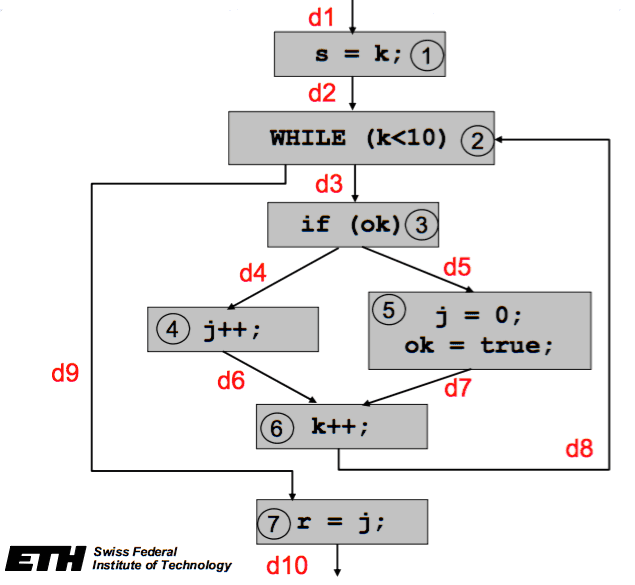
This image is taken from the lecture slides provided by Lothar Thiele.
Flow Equations (sum of incoming edges equals sum of outgoing edges)
Additional Constraints
- Execute the program only once:
- loop is executed at most 10 times:
- Block 5 is executed at most one time:
The more information the better the result
Integer Linear Program for WCET Calculation
ILP with structural and additional constraints
Abstract Interpretation (AI)
- Semantics-based method for static program analysis
- Basic idea
- Perform programs computations using value descriptions (or abstract values)
- Start with the description of all possible inputs
- AI supports correctness proofs
Ingredients:
- Abstract domain: related to concrete domain (by abstraction and concretization functions)
- e.g
- where:
- instead of:
- Abstract transfer functions: for each statement type (abstract versions of their semantics)
- e.g
- where:
- with: extends to
- A join function combining abstract values from different control-flow paths
- e.g
- where:
Value Analysis
Motivation:
- Provide access information to data-cache/pipeline analysis
- Detect Infeasible paths
- Derive loop bounds
Method:
Calculate intervals at all program points. Lower and upper bounds for the set of possible values occurring in the program (addresses, register contents, local and global variables).
Caches
-
Main memory to slow
-
Speed gap between CPU and memory too large (and increasing)
-
Caches work well in the average case:
- Programs access data locally (many hits)
- Programs reuse items (instructions, data)
- Access patterns are distributed evenly across the cache
-
Caches: fast, small, expensive
-
Memory: relatively slow (bottle neck), large, cheap
-
Access cycles:
- CPU ↔ Cache: ~1 cycle
- Cache ↔ Memory: ~100 cycles
How caches work:
- CPU wants to access (read/write) at memory address a
- Caches:
- Block m containing a is in the cache (hit):
- Request for a is served in next cycle
- Block m is not in the cache(miss):
- m is transferred from main memory to the cache
- m may replace some block in the cache
- Request for a is served as soon as possible (while transfer still continues)
- Several replacement strategies:
- LRU: Least Recently Used
- PLRU: Pseudo-LRU
- FIFO
- …
- Block m containing a is in the cache (hit):
Cache Analysis
Statically precompute cache contents:
- Must Analysis
- For each program point (and calling context) find out which blocks are in the cache
- Determines safe information about cache hits
- Predicted cache hit reduces WCET
- May Analysis
- For each program point (and calling context) find out which blocks may be in the cache
- Complement says what is not in the cache
- Determines safe information about cache misses
- Each predicted cache miss increases BCET
Must Cache
-
Only variables that are in all caches
-
Order: worst age (oldest)
-
Number of variables in cache numbers of places in cache
-
Join
- Intersection + maximal age
- Interpretation:
- Memory block a is definitely in the cache
- Always a hit
May Cache
- All variables that could be in cache
- Minimal age
- Join
- Union
- Minimal age
- Interpretation:
- All block may be in cache
- None is definitely not in cache
Cache Contribution to WCET
Reference to variable s in code:
- if s is in must-cache:
- otherwise
- if s is in may-cache:
- otherwise
Reference to variable s in loop body (max iterations):
-
First time miss, then always hit
-
Loop unfolding
-
within loop
Pipelines
- Different stages in parallel
- Fetch
- Decode
- Execute
- …
- Pipeline hazards
- Data hazard: Operands not yet available
- Resource hazard: Consecutive instructions use same resource
- Control hazard: Conditional branch
- Instruction-cache hazard: Instruction fetch causes cache miss
- CPU as State Machine: Abstract Pipeline for basic blocks
10 Performance Analysis of Distributed Embedded Systems
Embedded System = Computation + Communication + Resource Interaction
-
Analysis ↔ Design
- Analysis: infer system properties from subsystem properties
- Design: build system from subsystems while meeting requirements
-
Abstract model
| Concrete instance (real world) | Abstract representation (model) |
|---|---|
| Input stream | Load model |
| Processor | Service model |
| Task(s) running on processor | Processing model |
- System view
- Modular Performance Analysis (MPA)
- Mathematical view
- Real-Time Calculus (RTC)
- Min-Plus Calculus, Max-Plus Calculus
Real-Time Calculus
- Real-Time Calculus can be regarded as a worst-/best-case variant of classical queuing theory
- It’s a formal method for the analysis of distributed real-time (embedded) systems
Algebraic Structure
-
Set of elements
- One ore more operators defined on elements of this set
-
Algebraic structures with two operators: ,
- plus-times:
- Our ‘normal’ algebra
- min-plus:
- Used for Real-Time calculus
- plus-times:
-
Infimum
- The infimum of a subset (of some set) is the greatest element (not necessary in the subset) that is less than or equal to all other elements of the subset
- Examples:
- and
- but
-
Joint properties of :
- Closure:
- Associativity:
- Commutativity
- Existence of identity element:
- Existence of negative element:
- Identity element of absorbing for :
- Distributivity of w.r.t. :
-
Joint properties of :
- Closure:
- Associativity:
- Commutativity:
- Existence of identity element:
-
Differences :
- plus-times: Existence of negative element for :
- min-plus: Idempotency:
-
Example:
- plus-times:
- min-plus:
System Theories
- Plus-times system theory:
-
signals, impulse response, convolution, time-domain
-
: Signals
-
: Impulse response
-
: Convolution
-
: Time domain
-

- Min-plus system theory
-
streams, variability curves, time-interval domain, convolution
-
: Streams
-
: Variability curves
-
: Time-interval domain
-
: Convolution
-

From Streams to Cumulative Functions
- Event streams → Arrival Curves ()
- Event stream: number of events in
- Arrival Curves : maximum and minimum arriving events in any interval of length
- Resources → Service Curves ()
- Resource Availability: available service in
- Service Curves : maximum and minimum available service in any interval of length
- Arrival and Service Curves work on time intervals as domain ()
Overview of Methods and Algorithms
| Domain | Notes | |
|---|---|---|
| Hierarchical Clustering | Partitioning | |
| Integer Linear Programming | Partitioning | |
| Simulated Annealing | Partitioning | |
| Trace Based Simulation | Estimation | |
| Evolutionary Algorithms | Partitioning | Multi Objective Optimization |
| Tom Parks Algorithm | Kahn Process Networks | |
| Kerninghan Lin | Partitioning |